Multi-DOF Robotic Manipulator Project

📄 Full Project Documentation

You can access the full documentation here.

Project Overview: Multi-DOF Robotic Manipulator

This project presents the complete engineering lifecycle of a multi-degree-of-freedom (Multi-DOF) robotic manipulator, transitioning from mathematical kinematic modeling to a functional physical prototype. The objective was to bridge theoretical robotics with practical application by designing a system capable of precise, real-time motions.

System Configuration and Design

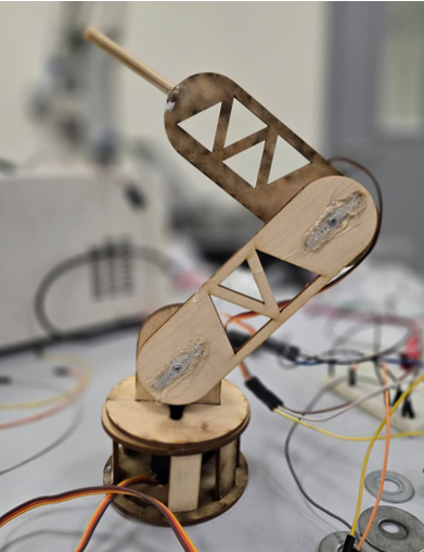
Manipulator Structure: 3-DOF planar configuration consisting of one base rotation joint, two serial revolute joints, and two rigid links.
Mechanical Fabrication: Structural components were designed in CAD and fabricated using laser cutting from 3 mm plywood.
Link Specifications: First link (L_1 = 0.14\,\mathrm{m}), second link (L_2 = 0.12\,\mathrm{m}).
Control Hardware: Arduino Uno interfaced with three servo motors for joint actuation.

Technical Methodology

Kinematic Modeling: Denavit–Hartenberg (DH) convention was used to derive homogeneous transformation matrices relating joint variables to the end-effector’s pose.
Simulation: MATLAB Robotics Toolbox validated the manipulator prior to assembly. Functions like fkine() and teach() ensured algorithmic correctness.
Verification: Tinkercad was used to pre-validate wiring and motion logic.

Core Mathematical Framework

1. Forward Kinematics (2-DOF Planar)

The end-effector ((x, y)) position based on joint angles (\theta_1) and (\theta_2):

\[\begin{aligned} x &= L_1 \cos(\theta_1) + L_2 \cos(\theta_1 + \theta_2) \\ y &= L_1 \sin(\theta_1) + L_2 \sin(\theta_1 + \theta_2) \end{aligned}\]

2. Homogeneous Transformation Matrix

Using the DH convention, the individual transformation matrix for link (i) is:

\[A_i = \text{Rot}_{z, \theta_i} \, \text{Trans}_{z, d_i} \, \text{Trans}_{x, a_i} \, \text{Rot}_{x, \alpha_i}\]

3. Inverse Kinematics (3-DOF Geometric Approach)

For a target position ((x, y, z)), the 3D problem reduces to a 2D (k-z) plane.

Base Angle: \(\theta_1 = \tan^{-1}\frac{y}{x}\)
Elbow Angle ((\theta_3)) using the law of cosines: \(\theta_3 = -\cos^{-1}\frac{x^2 + y^2 + z^2 - L_1^2 - L_2^2}{2 L_1 L_2}\)
Shoulder Angle ((\theta_2)): \(\theta_2 = \sin^{-1}\frac{z}{r} + \tan^{-1} \frac{L_1 + L_2 \cos\theta_3}{L_2 \sin\theta_3}, \quad r = \sqrt{x^2 + y^2 + z^2}\)